Starting RL: Markov Decision Process in plain english

A Markov Decision Process is one of the most fundamental knowledge in Reinforcement Learning. It’s used to represent decision making in optimization problems.

The version we present here is the Finite MDP, which analyses discrete time, with discrete action problems, with some amount of stochasticity involved. This means the same sequence of actions has a probability to lead to a different situation between two tries.

Here, we focus on the presenting a general structure of the mathematical framework, such as the elements involved and the equations linking them together. We’ll also cover some difficulties we might encounter when formulating a problem as an MDP.

---

Interactions between an agent and the environment

Your learning system is often called an agent, in most modern literature. This term includes more than just the neural network estimator in recent algorithms. The agent interacts with an environment to solve a task. We’ll go into further details later into what constitutes the environment, as it can become problematic. The environment relies on two main components: its transition and reward functions. Both are linked to the nature of the system and of the task.

For example, the following graph represents an environment with three states and four actions available to an agent. The task the agent must accomplish is transitioning all three states and coming back. There are states with positive and negative rewards, which could correspond to marginal gain or detrimental side-goals. This view is from an external, omnipotent observer, that can see the problem as a whole. This is generally not the case for our agents, that can only observe what’s around them and the result of their direct actions.

The graph representation is a visual synthesis of the MDP, expressed as a tuple:

Where:

• is the set of all states reachable by the agent. They are the blue nodes in the previous graph.
• is the set of actions, called the action space. This is often conditioned by the state , meaning the actions available in that state s. They are the orange nodes in the previous graph.
• is the transition probability matrix. It corresponds to the probabilities that an action a will transition state s to state s’. They are the probabilities noted after some actions in the previous graph, such as 0.6 to transition from state 2 to state 1 after using action 1.
• is the immediate reward resulting from a transition between s and s’. They are denoted by integers pointed to by a red squiggle.

While the graph is a representation of the whole system, if we want to analyse an agent’s experience, we must describe each decision within its context. This context is generally within an episode, a finite sequence from t=0 to T.

The length of an episode is generally defined by the task, such as solving a maze in Y moves. But, some problems are potentially infinite, with no tractable end in sight, such as in financial trading or low-level robotics. In this case, an episode’s end is defined artificially, and the agent learns on a segment of the experience.

Each interaction is defined as the tuple:

From the current state s, the agent chooses action a, which leads to the new state s’, with the reward r. The action was chosen based on a policy π, the main component your learning algorithm is trying to optimize in any approach of RL.

The policy π is a mapping between a state representation and actions. We have a similar behavior, as humans: when going home, we know to turn left on a specific intersection, or to hit the brakes when a traffic light turns red. We recognize patterns and know which actions match them.

But, to recognize something, it needs a distinct shape, which allows us to make the right decisions. If all the corridors in a building were exactly the same, with no signage, would you be able to find your way around using only what your eyes saw at a given moment?

---

Representing the system

The main purpose of a state representation is giving an agent enough information for it to know which state it is in and where it should go next. These could include sensor readings, images or processed indicators.

In tasks where only observations are needed, such as for a robotic arm picking up an object, only the sensors are required. If we know where the arm and the object are, we can predict increments for the rotors.

In tasks that require some notion of history, processed indicators are necessary. In a self-driving car, sensing the position of a car is as important as knowing where that car is going.

In both cases, the proper granularity of information is important. Any granularity suitable for the task can be used, from the lowest sensors to the highest abstraction level.

Telling a robotic arm that it must go “left”, when it controls rotors, may not be enough: how far must it go? 1 increment, a quarter turn or a full turn? It must be adapted to each task, to facilitate the agent’s learning.

As such, a controller agent may be trained to give out high-order actions, such as “left, right, down, up”, that a driving agent may interpret as input. This driving agent will then, in turn, act upon rotors using low-level actions such as voltage or increments.

Robotics problems highlight another preoccupation: where do we define the split between an agent’s properties and the environment? The absolute position of an arm in a space or the amount of stock in inventory gives agents important information about the environment, but are linked to their actions, which should be part of the agent and not the environment.

Yet, they are the results of the actions, either from applying a voltage to motors or from buying items. The limit between the agent and the environment are the variables directly under control of the agent. As such, the last voltage applied should not be considered part of the environment, but as part of the agent.

---

Creating your goals

The goal of an agent is to maximize the expected rewards from a sequence of actions. As the expected rewards are the cumulative score achieved through a whole episode, the agent may make locally sub-optimal choices, in order to reach more profitable results later on. This is most evident in the game of chess, where players are willing to sacrifice pieces, if it leads to a favorable position. What is considered favorable or otherwise is defined by the reward function.

Rewards

A reward is given for specific state-transitions. They can be reached either at every step or at the end of an episode. Since an agent tries to maximize them, properly shaping a reward function can influence the desired behavior we wish to see an agent display. It can be any value function as long as it highlights the desired end goal.

1. For tasks with clear end-goals, a large reward can be given when it is reached.
2. For video games, the in-game score can be exploited.
3. Yet for robotics tasks with safety preoccupations, we also need a way to discourage dangerous behavior.
   • If the safety of humans is at risk, ending an episode early with a large negative reward ensures the agent quickly steers away from these actions.
   • For less severe cases, negative rewards ensure that the agent does not dwell in that state.

Rewards can include a combination of different functions as long as it respects fundamental metrics guidelines. As such, it should be convex, so that given an order, you are able to rank performances using that order. If a greater score is better, there should not be any circumstances where a lower score reaches a better ranking.

Finally, while using composite functions, they should all be on the same order of magnitudes or the lower order functions will rarely be taken into account.

Returns

We define the returns G as the cumulative rewards which our agent receives during an episode:

In many RL problems, the length of episodes are quite long. As such, the first steps in an episode may have confusing expected returns, with no clear actions to make. One solution was to introduce a discounting factor. It narrows how far ahead an agent estimates the rewards it can reach. Our return G becomes:

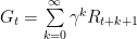
As we can see, selecting a proper means that steps further out contribute close to nothing to an actions’ returns:

Therefore, the expected returns from a given time within an episode can be obtained from:

For reference, here is a scale of how far ahead the agent can look based on :

• 0.9 = 10 steps
• 0.99 = 100 steps
• 0.999 = 1000 steps

---

Defining the maths behind MDP

From previous sections, we have seen the transition probability matrix, and how to compute the expected returns from an episode. These notions are the basis that allow us to conceive the building blocks of a decision making process!

We can estimate the returns we can reach by using any action in our current state:

The current state s is fixed, so we can iterate all the actions a available in s. For each action, we estimate the probability of landing in state s’, which should reward us with a score r. In many problems, the function Pr is known, but for others, it is estimated using techniques such as Monte Carlo Sampling.

From this equation, we can also disregard the rewards and focus on the state-transition probabilities, where we are likely to go next:

To obtain only the expected returns, for each path available to the agent in its state, we use the “state — action — next state” estimated returns:

---

The Markovian Property and Why it matters

This normally requires more than the immediate sensations, but never more than the complete history of all past sensations.

Sutton and barto, 2018

The Markovian Property is a requirement for what is included in the state signal, which completes what was mentioned in the “Representing the System” section.

The information must only contain a sense of immediate measurements. Keeping all past observations is highly discouraged due to the intractability of such a practice. But, a sense of past actions, such as to highlight movement in an autonomous car system, is possible. The idea is to keep the picture as light as possible to facilitate learning a policy π.

This property is required because the mathematical framework assumes that the next state s’ is directly linked to the current state s and the action a that was chosen. If this relation is not true, the main equations fail and learning becomes unlikely.

However, perfectly Markovian problems are rare in the real world, which is why some tolerance is accepted, and newer frameworks, including Partially Abstract MDP and Partially Observable MDP (POMDP), were presented in recent years.

These have allowed us to model problems including Poker, which is famous for being an incomplete problem, where each player has no information about its opponent’s hand. It is also made more complex by the psychology involved in the game. A player may be known to bluff frequently, or to fold when unsure.

Thus, Poker requires information which is not available in the direct environment, and therefore contradicts the Markovian Property. Yet, we have seen some recent results of Deep Reinforcement Learning agents beating Human Poker players. This depends on framing the problem and finding a way to convey enough information to the agent.